When I first started learning about neural networks, I found it very difficult to match the math to the code. Most papers and explanations merged the math that's required for neural networks with the math that's an optimization. It made it very difficult to piece out exactly what was needed to make it work at all vs what was needed to make it work faster.
This book will build up the math and code for neural networks side by side, starting with the smallest neural network possible.
By the end of this first chapter, you will:
That's right! By the end of this chapter you'll have derived and understood the calculus that makes neural networks work, and you'll have written a neural network library based on that exact same math.
If you haven't already, sign up at https://www.milestonemade.com/building-with-neurons/ to be notified when new chapters are available.
A neural network is a graph of single neurons, and each neuron is just small math formula. The output of some neurons is fed as input to other neurons. Mathematically, this means that a neural network is a composition of math formulas.
\[ \newcommand{\alignThreeEqs}[4][=]{{#2} #1 & {#3} & #1 {#4}\\}\newcommand{\alignTwoEqs}[3][=]{#2 & #1 & #3\\} N = n_2(n_1(\text{input})) = \text{prediction} \]
Surprisingly, the coefficients in each neuron's formula are initialized to completely random numbers. Unsurprisingly, this means the initial output of a neural network is completely random as well! In order for a neural network to make accurate predictions, it needs to be trained - its neurons' coefficients need to be updated.
Input/output pairs of training data are used to train the network by comparing its prediction for a given input to the correct value. An error value is calculated from the difference, and this error value is used to gently update the neuron formula's coefficients through a process called backpropagation.
This chapter explains the bare minimum necessary to translate the math of neural networks 1:1 into code. Our goal today is clarity. We're not trying to build an F1 race car; we're not even trying to build a Model T. We're trying to build a tiny two-stroke lawnmower engine.
By the end of this chapter, you'll have built the smallest possible neural network, derived the math for backpropagation, and implemented all of it into code. Most importantly, you'll understand why it all works!
I think we've set ourselves a very reasonable goal: we want to define the smallest possible neural network. There's no smaller network than just 1 neuron! And since individual neurons are essentially just math formulas, what's the simplest formula that has at least 1 input and 1 output? A line!
\[y = ax + b\]
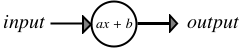
Perfect! Let's use that for our single neuron! Our simple network will take in a single input and provide a single output:
Let's rewrite this formula using the jargon of neural networks. Instead of calling \(a\) and \(b\) coefficients, we'll use \(w_1\) and \(w_2\) for "weight." And instead of \(y\), the output of a neuron is typically called its "activation," so we'll use that term as well.
\[ \begin{eqnarray*} \alignTwoEqs{y}{activation} \alignTwoEqs{a}{w_1} \alignTwoEqs{b}{w_2} \alignTwoEqs{x}{input} \alignTwoEqs{activation}{w_1 \times input + w_2} \end{eqnarray*} \]
Before our neuron can predict anything, we'll need to initialize our formula with some weights. If you're anything like me, this might make you a bit uncomfortable: we're just going to pick small random numbers to assign to \(w_1\) and \(w_2\) - yikes! Trust me this'll work out. Neural network software automatically initializes weights randomly, but we'll do it manually so we can see exactly what's happening. Let's pick 0.1 and 0.2.
\[ \begin{eqnarray*} \alignTwoEqs{w_1}{0.1} \alignTwoEqs{w_2}{0.2} \alignTwoEqs{activation}{w_1\times input + w_2} \end{eqnarray*} \]
So let's get coding! Well, pseudo-coding. The pseudocode in this book will be easy enough to read for you to translate into your language of choice.
class Neuron{
    property input
    property activation
    property weights = [0.1, 0.2]

    function feedForward(){
        activation = weight[0] * input + weight[1]
    }
}
Note: our code indexes the weights starting with 0, but most books and academic papers use 1-indexing, so we'll start our formulas with 1 as well. It's a small detail, but something to keep in mind as we match the math to code.
Even though we've initialized our neuron with a completely random formula for a line, we're expecting and hoping that this neuron will be able to learn and predict something that's not random.
This also means that the neuron's formula will change over time. Since our neuron models the formula \(ax+b\), training must change either \(a\), \(x\), or \(b\). But \(x\) is provided as our input - the only values available for us to change inside the neuron are \(a\) and \(b\)! So it's only these weights that are allowed to change during training.
Now that we can train our neuron, we need some data to train with!
So we've built our neuron - but what exactly are we going to predict? Well, a neuron that uses the formula for a line should be pretty good at predicting linear data, so let's train our network to predict the corresponding Fahrenheit temperature for an input Celsius temperature.
\[F = 1.8 \times C + 32\]
In code, that'd look like:
function convertCtoF(testInput){
    return 1.8 * testInput + 32
}
Perfect, now we can easily generate a piece of test data by picking a random number and running it through our new function:
testX = random() % 20 - 10 // pick between -10 and 10
testY = convertCtoF(testX)
This will make it very easy to generate test data without needing to pre-define a huge table of data.
At this point, we have the math and code for our single-neuron neural network and our test data. It's time to ask our network for its first prediction.
Our neuron:
\[ \begin{eqnarray*} \alignTwoEqs{w_1}{0.1} \alignTwoEqs{w_2}{0.2} \alignTwoEqs{activation}{w_1\times input + w_2} \end{eqnarray*} \]
Sending our network an input and calculating a prediction is called feedforward. This step is particularly simple for our case since our network is composed of only a single neuron. For our feedforward step, we calculate the activation of our neuron for a given input. Let's find out what our network would predict for the ℉ value of 17℃.
\[1.9℉ = 0.1 \times 17℃ + 0.2\]
In code, that'd look like:
n = new Neuron()
n.input = 17

prediction = n.feedForward()
print prediction // 1.9
Ok, 1.9℉ is definitely not the correct Fahrenheit value for 17℃, but just how wrong is it? Is it a lot wrong? or just a little?
To know that, we need to formalize how we calculate our error for a given prediction, and then how we can use that error measurement to help our network learn.
In order for us to train our neural network, the last thing we need to define is our error formula. We need to know how wrong our network is after each activation, and since it's been randomly initialized, I suspect it will be very wrong. We saw above that our network predicts that 17℃ is 1.9℉, but what's the real temperature?
\[ \begin{eqnarray*} \alignTwoEqs{F}{1.8 \times C + 32} \alignTwoEqs{62.6}{1.8 \times 17 + 32} \end{eqnarray*} \]
Yep! Definitely wrong! Just how wrong was our network? Let's define our rate of error as:
\[ \begin{eqnarray*} \alignTwoEqs{error}{goal - activation} \alignTwoEqs{60.7}{62.6 - 1.9} \end{eqnarray*} \]
Great! That gives us a measured error of 60.7. And since our network is so simple, we can even graph our measured error rate for any input.
\[ \begin{eqnarray*} \alignTwoEqs{error}{goal - activation} \alignTwoEqs{error}{(1.8 \times C + 32) - (0.1 \times C + 0.2)} \alignTwoEqs{error}{1.7 \times C + 31.8} \end{eqnarray*} \]
Let's graph that and see what we're working with:
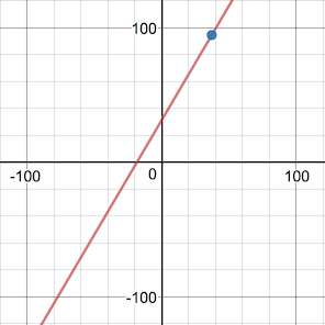
Ok, that's odd, the error dips below 0 on the left hand side. When we predict ℃ for an input of -40℉, we get a negative error:
\[-36.2 = 1.7 \times -40 + 31.8\]
What does it even mean to have a negative error? Intuitively, a positive error makes sense: the larger the error the more wrong our prediction is. In the same way, we expect that the more negative our error is, the more wrong we are.
\[ \begin{eqnarray*} \alignTwoEqs{error_{simple}}{goal - activation} \alignTwoEqs{error}{\big|error_{simple}\big|} \end{eqnarray*} \]
Perfect, now our error measure will always be positive, which makes more sense. The further away our prediction is from reality, the larger the error. If we had asked to predict with -18.7℃, then our neuron would have correctly predicted -1.66℉ with 0 error.
In the graph below we see the error line hit 0 at -18.7℃.
Let's update our code:
class Neuron{
    property input
    property activation
    property weights = [0.1, 0.2]

    function feedForward(){
        activation = weight[0] * input + weight[1]
    }

    function simpleErrorFor(goal){
        return goal - activation
    }

    function errorFor(goal){
        return ABS(simpleErrorFor(goal))
    }
}
Next up: training! When we train, we'll be trying to reduce the network's error as close to zero as possible. We saw above that we can get 0 error for one specific input, training will help us drive toward 0 error for all inputs. We want that error graph to be as flat on the X axis as possible.
Ok, we're getting very very close to the magic now! Let's get all of our formulas in one place. We'll use \(w_1\) and \(w_2\) to represent the two weights in our neuron.
\[ \begin{eqnarray*} input & = & 17℃ \\ goal & = & 62.6℉ \\ \\ activation & = & w_1 \times input + w_2 \\ & = & 0.1 \times 17 + 0.2 \\ & = & 1.9 \\ \\ error & = & \big|goal - activation\big| \\ & = & \big|62.6 - 1.9\big| \\ & = & 60.7 \\ \end{eqnarray*} \]
There appears to be a surprising number of moving parts to this very simple neural network! We have:
Remember, there's only one piece of this puzzle that we can change during training - the weights. Let's take a second look at activation and error formulas, defining them in terms of \(w_1\) and \(w_2\). With the constants filled in and using \(a\) for activation and \(e\) for error, we get:
\[ \begin{eqnarray*} a(w_1, w_2) & = & w_1 \times 17 + w_2\\ e(a) & = & \big|62.6 - a\big| \end{eqnarray*} \]
Activation is a function with weights as input, and error is a function with activation as input. And now we see we can substitute the activation formula into the error formula!
\[ \begin{eqnarray*} e(w_1, w_2) & = & \big|62.6 - (w_1 \times 17 + w_2)\big| \end{eqnarray*} \]
Holding each of the weights constant, we can define our error in terms of each weight:
\[ \begin{eqnarray*} e_{w1} & = & \big|62.6 - (w_1 \times 17 + 0.2)\big|\\ e_{w2} & = & \big|62.6 - (0.1 \times 17 + w_2)\big|\\ \end{eqnarray*} \]
Let's simplify these a bit:
\[ \begin{eqnarray*} e_{w1} & = & \big|62.4 - w_1 \times 17\big|\\ e_{w2} & = & \big|60.9 - w_2\big| \end{eqnarray*} \]
This means that we can now see how each weight affects error! This is different than the error graph in the previous section. There we graphed how error changed as we changed the input. Here, we're holding the input constant to see how changing each weight affects the error.
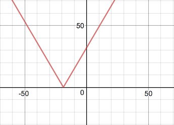
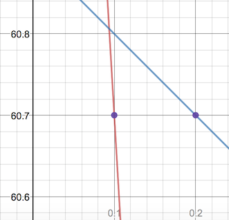
What can we learn when we graph these? I've plotted \(e_{w1}\) in red and \(e_{w2}\) in blue below, with the purple dot showing total error \(e(.1, .2)\):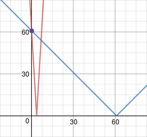
It might look like our current error is at the exact intersection of the two lines - but that's an artifact of the graph's zoom. If we zoom in, it'll be clear what's happening: the \(e_{w1}\) error is at \(w_1 = .1\), and the \(e_{w2}\) error is at \(w_2 = .2\).
\[ w_1 = .1\\ w_2 = .2\\ \begin{eqnarray*} \alignThreeEqs{ e_{w1} }{ \;\big|62.4 - w_1 \times 17\big| }{ 60.7 } \alignThreeEqs{ e_{w2} }{ \big|60.9 - w_2\big| }{ 60.7 } \end{eqnarray*} \]
Having exact equations like this means that we can solve for \(e = 0\) directly! When we do that, we see that setting either \(w_1 \approx 3.7\) or \(w_2 = 60.9\) will reduce our error to zero.
Let's try it out and test updating a weight to one of these roots. Using the new value for \(w_2\), our neuron would look like:
\[ \begin{eqnarray*} w_1 & = & 0.1\\ w_2 & = & 60.9\\ activation & = & w_1 \times input + w_2 \end{eqnarray*} \]
Which would make our activation for that sample input:
\[ \begin{eqnarray*} activation & = & 0.1 \times 17 + 60.9\\ & = & 1.7 + 60.9\\ & = & 62.6 \;\;\;\text{(!)}\\ \end{eqnarray*} \]
Look at that! We've "corrected" our answer by updating just one of our weights and accurately predicted 17℃ is 62.6℉! Unfortunately, our neuron would still be wrong for every other input - it's only corrected for that single input. Let's look at the graph of what our neuron predicts (green) for ℃ inputs vs the true formula (purple).
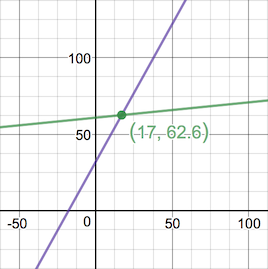
The graph makes it obvious that we'll only correctly predict that single input of 17℃. And even looking at the formulas it's clear they won't behave the same.
\[ \begin{eqnarray*} our\space neuron & = & 0.1 \times input + 60.9\\ reality & = & 1.8 \times input + 32\\ \end{eqnarray*} \]
What we'd really like to see after training our neuron on many test cases is:
\[ \begin{eqnarray*} w_1 & \approx & 1.8\\ w_2 & \approx & 32\\ our\space neuron & \approx & 1.8 \times input + 32\\ \end{eqnarray*} \]
It's obviously not enough to train by just using the root values of that error graph. If we just change \(w_2\) over and over again, we'll just be shifting that red line up and down. And if we only change \(w_1\) over and over, then we'll just be rotating our line around the point (0, \(w_2\)). We need our training to shift and rotate our red line into position to overlap the blue line.
Let's try a different approach and see what else these error formulas are telling us.
Let's look at the \(e_{w1}\) and \(e_{w2}\) graphs again.
Notice that for both \(e_{w1}\) and \(e_{w2}\) formulas, both error lines have negative slopes at their input weights. What if we move the weights to the right along those lines? If we increase both values, it should decrease the error!
So let's try something different. Instead of correcting one weight a lot, let's try correcting both weights just a little:
\[ \begin{eqnarray*} bump & = & 0.1\\ w_1 & = & 0.1 + bump\\ w_2 & = & 0.2 + bump\\ activation & = & w_1 \times input + w_2\\ & = & 0.2 \times 17 + 0.3\\ & = & 3.4 + 0.3\\ & = & 3.7\\ \end{eqnarray*} \]
We still didn't predict the correct answer of 62.6, but our new activation of 3.7 is definitely better than the original activation of 1.9! Our neuron still isn't accurate, but it's certainly more accurate!
Look again at the \(e_{w1}\) and \(e_{w2}\) graphs above. If we bump \(w_1\) even a tiny bit, we can see that the error will change dramatically! Similarly, if we change \(w_2\) by the same amount, the error won't change nearly as much. That's the clue we're looking for! We want to bump each weight according to how much it would affect the error! The steep slope of \(e_{w1}\) and more shallow slope of \(e_{w2}\) are our clues for how much to adjust each weight.
This is the essence of how neural networks learn. Do this lots of times for lots of input/output pairs, bumping the weights just a bit each time, and voilà! The network has learned!
We're so close! We know why we should bump each weight, and we know what direction to bump each weight, but we still don't know exact formulas for how much to bump each weight. In the above example, I chose 0.1, but that's hardly scientific. Instead we should somehow be using the slope of the error function.
This is our next challenge, and this is where the magic of neural networks really comes alive! And by "magic," I mean "calculus." And by "calculus," I mean "it's not as bad as it sounds." Let's use calculus magic with these error graphs to determine how much we should bump each weight. To do that, we'll need to find the derivatives of the \(e_{w1}\) and \(e_{w2}\) functions.
The slope of a line tells us how much that line changes vertically for every step horizontally. It's a measure of rate of change for that line, and that's exactly what the derivative of a formula tells us. For a formula \(f(x)\), the derivative \(f'(x)\) tells us how fast or slow the value of \(f(x)\) is changing at that \(x\).
For our purposes, we only need to remember a few key specifics about derivatives. First, the derivative of \(|x|\) is:
\[ \begin{eqnarray*} \frac{\partial}{\partial x} |x| = \begin{cases} -1 & x\lt 0 \\ 1 & x\gt 0 \\ \end{cases}\\ \end{eqnarray*} \]
We'll also need to remember the Chain Rule:
\[ \begin{eqnarray*} \frac{\partial f}{\partial x} = \frac{\partial f}{\partial g}\frac{\partial g}{\partial x} \end{eqnarray*} \]
or put another way:
\[ \begin{eqnarray*} F(x) & = & f(g(x))\\ F'(x) & = & f'(g(x))g'(x) \end{eqnarray*} \]
Bringing these two together, we get:
\[ \begin{eqnarray*} \frac{\partial}{\partial x} |g(x)| & = & g'(x) & \begin{cases} -1 & g(x)\lt 0 \\ 1 & g(x)\gt 0 \\ \end{cases}\\ \end{eqnarray*} \]
We saw in the previous section that the error of our neuron is simply a function of its weights, \(e(w_1, w_2)\). We also saw that to minimize the error, we should move in the opposite direction of \(e_{w1}\) and \(e_{w2}\)'s slope. When the slope of the line is negative, we should increase that weight. And when the slope is positive, we should decrease that weight. Using this process to update our neuron's weights is called backpropagation.
Let's try using the \(e(w_1, w_2)\) function's derivative with respect to each weight to help us determine how much we should move down the slope.
Let's start with our error and activation formulas. It'll also be helpful for us to separate out \(e_{simple}\) from the absolute value in \(e\):
\[ \begin{eqnarray*} \alignTwoEqs{ a(w_1, w_2) }{ w_1 \times input + w_2 } \alignTwoEqs{ e_{simple}(a) }{ goal - a } \alignTwoEqs{ e_{abs}(e_{simple}) }{ \big|e_{simple}\big| } \end{eqnarray*} \]
We now see that our total error is the composition of these three functions.
\[ error = e_{abs}(e_{simple}(a(w_1, w_2))) \]
Conveniently, we just reviewed the Chain Rule to help us calculate this exact sort of derivative! So we know that:
\[ \frac{\partial e}{\partial w} = \frac{\partial e_{abs}}{\partial e_{simple}} \frac{\partial e_{simple}}{\partial a} \frac{\partial a}{\partial w} \]
Let's solve for those derivatives:
\[ \begin{eqnarray*} \alignThreeEqs{ \frac{\partial e_{abs}}{\partial e_{simple}} }{ \frac{\partial}{\partial e_{simple}}\big|e_{simple}\big| }{ \begin{cases} -1 & e_{simple}\lt 0 \\ 1 & e_{simple}\gt 0 \\ \end{cases} }\\ \alignThreeEqs{ \frac{\partial e_{simple}}{\partial a} }{ \frac{\partial}{\partial a} (goal - a) }{ -1 }\\ \alignThreeEqs{ \frac{\partial a}{\partial w_1} }{ \frac{\partial}{\partial w_1}(w_1 \times input + w_2) }{ input }\\ \alignThreeEqs{ \frac{\partial a}{\partial w_2} }{ \space\space \frac{\partial}{\partial w_2}(w_1 \times input + w_2) }{ 1 } \end{eqnarray*} \]
Now we can solve for \(e\)'s derivative with respect to each weight! This will tell us how much each weight is responsible for the error.
\[ \begin{eqnarray*} \\ e_{w1}'(e_{simple}) & = \alignThreeEqs{ \frac{\partial e}{\partial w_1} }{ \left(\begin{cases} -1 & e_{simple}\lt 0 \\ 1 & e_{simple}\gt 0 \\ \end{cases}\right)(-1)(input) }{ \begin{cases} input & e_{simple}\lt 0 \\ -input & e_{simple}\gt 0 \\ \end{cases} } \\ e_{w2}'(e_{simple}) & = \alignThreeEqs{ \frac{\partial e}{\partial w_2} }{ \left(\begin{cases} -1 & e_{simple}\lt 0 \\ 1 & e_{simple}\gt 0 \\ \end{cases}\right)(-1)(1) }{ \begin{cases} 1 & e_{simple}\lt 0 \\ -1 & e_{simple}\gt 0 \\ \end{cases} } \end{eqnarray*} \]
Since we want to move the opposite direction of the slope of the error, we'll want to subtract this derivative from each weight. Every time we train a new ℃/℉ pair, we'll subtract \(e_{w1}'\) from \(w_1\) and \(e_{w2}'\) from \(w_2\).
\[ w_{1 \space next} = w_{1} - e_{w1}'(e_{simple})\\ w_{2 \space next} = w_{2} - e_{w2}'(e_{simple}) \]
With our new knowledge of the error derivative formulas with respect to each weight, let's look again at the graph for simple error and see what this means graphically. We can see clearly below that our slope for \(e_1\) is steeper than for \(e_2\), so our adjustment to \(w_1\) should be larger than our adjustment to \(w_2\).
Since \(e_{simple}\) is positive, we can now calculate \(w_{1 \space next}\) and \(w_{2 \space next}\).
\[ \begin{eqnarray*} input & = & 17\\ e_{simple} & = & 60.7\\ e_{w1}' & = & -input = -17\\ e_{w2}' & = & -1 \end{eqnarray*} \]
\[ \begin{eqnarray*} \alignThreeEqs{ w_{1 \space next} }{ \;w_{1} - (-input) }{ 17.1 } \alignThreeEqs{ w_{2 \space next} }{ w_{2} - (-1) }{ 1.2 } \end{eqnarray*} \]
And thankfully, we do see that \(e_{w1}'\) is steeper than \(e_{w2}'\), so our math seems to be matching our expectations.
Let's translate everything we just did into code! I find that the math always makes much more sense to me once I can see it operate in code, and compute step by step.
We'll update our Neuron class below:
class Neuron{
    property input
    property activation
    property weights = [0.1, 0.2]

    function feedForward(){
        activation = weights[0] * input + weights[1]
        return activation
    }

    function backpropagate(goal){
        e_simple = simpleErrorFor(goal)
        delta_w0 = errorDerivativeForWeight0(e_simple)
        delta_w1 = errorDerivativeForWeight1(e_simple)

        // subtract the derivative to move _opposite_ the slope
        weights[0] -= delta_w0
        weights[1] -= delta_w1
    }

    function simpleErrorFor(goal){
        return goal - activation
    }

    function errorFor(goal){
        return ABS(simpleErrorFor(goal))
    }

    function errorDerivativeForWeight0(e_simple){
        e_deriv = (e_simple < 0) ? -1 : 1
        e_simple_deriv = -1
        a_deriv = input
        return e_deriv * e_simple_deriv * a_deriv
    }

    function errorDerivativeForWeight1(e_simple){
        e_deriv = (e_simple < 0) ? -1 : 1
        e_simple_deriv = -1
        a_deriv = 1
        return e_deriv * e_simple_deriv * a_deriv
    }
}And now, at long last, we can train our neuron!
n = new Neuron()

for(iter = 1 ... 3600){
    celsius = random() % 20 - 10
    fahrenheit = 1.8 * celsius + 32

    n.input = celsius
    n.feedForward()
    n.backpropagate(fahrenheit)

    error = n.errorFor(fahrenheit)
    avgError = avgError * 0.99 + abs(error) * 0.01

    log("Asked for %℃ => %℉. Predicted %℉. Error %", celsius, fahrenheit, n. activation, error)

    if(avgError < .25){
        log("Error is less than 0.25 degrees at iteration %", iter)
        break
    }
}
Uh oh! It doesn't seem to be working. Instead of getting more accurate, our neuron is spiraling out of control! Its predictions are getting worse and worse.
There's one last piece for us to implement to get our neuron behaving properly!
Let's pull up the graph of our error functions one more time. The red line, \(e_{w1}\), has a very large slope, so a very small change in \(w_1\) will produce a huge change in the weight.
This dramatic change in the weight will produce a large change in our predictions too. But remember our experiment where we bumped the neuron's weights? We were making only tiny changes to the weights to improve the prediction, but the slope of our lines is a much larger number in comparison.
Instead of using the full magnitude of the slope to update the weight, we should try scaling it to ensure its a very small bump to the weight. It turns out that the exact value of each slope is much less important than the relative slopes of the error lines. It's more important that \(e_{w1}' > e_{w2}'\) than it is that \(e_{w1}'\) is a large number.
Let's update our Neuron code on the following page and add in a learning rate.
With our new learning rate implemented, it's time to train again! This time you should see the weights converge to match the correct formula. After 3600 iterations, the neuron will predict within just \(\frac{1}{4}\)℉ of the correct value!
In the next chapter, we'll look at how different error formulas affect our math and our neuron's training speed.
class Neuron{
    property input
    property activation
    property weights = [0.1, 0.2]
    property learningRate = 0.01

    function feedForward(){
        activation = weights[0] * input + weights[1]
        return activation
    }

    function backpropagate(goal){
        e_simple = simpleErrorFor(goal)
        delta_w0 = errorDerivativeForWeight0(e_simple)
        delta_w1 = errorDerivativeForWeight1(e_simple)

        // subtract the derivative to move _opposite_ the slope.
        // use learningRate to ensure _small_ bump
        weights[0] -= learningRate * delta_w0
        weights[1] -= learningRate * delta_w1
    }

    function simpleErrorFor(goal){
        return goal - activation
    }

    function errorFor(goal){
        return ABS(simpleErrorFor(goal))
    }

    function errorDerivativeForWeight0(e_simple){
        e_deriv = (e_simple < 0) ? -1 : 1
        e_simple_deriv = -1
        a_deriv = input
        return e_deriv * e_simple_deriv * a_deriv
    }

    function errorDerivativeForWeight1(e_simple){
        e_deriv = (e_simple < 0) ? -1 : 1
        e_simple_deriv = -1
        a_deriv = 1
        return e_deriv * e_simple_deriv * a_deriv
    }
}