In the last chapter, we saw how gently bumping the weights of our neuron would train the neuron toward the correct answer. To find how much to bump each weight, we calculated the total error as the difference between our desired output and our actual output, and we then calculated the derivative of our neuron's formula to assign some of that error to each weight. The formal name for this measure of error is the mean absolute error (MAE). Error functions are also called cost functions or loss functions.
Let's take a look at the weights' error formulas again.
\[ \newcommand{\alignThreeEqs}[4][=]{{#2} \, #1 \, & {#3} & \, #1 \, {#4}\\} \newcommand{\alignTwoEqs}[3][=]{#2 & \, #1 \, & #3\\} \begin{eqnarray*} \alignTwoEqs{ e_{w1}'(e_{simple}) }{ \begin{cases} input & e_{simple}\lt 0 \\ -input & e_{simple}\gt 0 \\ \end{cases} } \\ \alignTwoEqs{ e_{w2}'(e_{simple}) }{ \begin{cases} 1 & e_{simple}\lt 0 \\ -1 & e_{simple}\gt 0 \\ \end{cases} } \end{eqnarray*} \]
Notice that the amount we change each weight depends on two things:
Notably, the size of a weight's adjustment does not depend on the size of our error! The adjustment to the weights depends on the slope of the error, not its magnitude. This means that very large errors are having the same sized effect on our neuron as very small errors.
In this chapter we'll be learning about the Mean Squared Error, which adjusts each weight proportionally based on how much each weight contributed to the neuron's error.
As an example, imagine that a criminal gang is captured and charged for various crimes they have committed. The leader (\(e_{w1}'\)), who bears more responsibility, will be punished more harshly than a low-level member (\(e_{w2}'\)) who was less involved, and the size of their punishment will rise if more serious crimes were committed (\(e_{simple}\)). Similarly, for our neuron, very large mistakes deserve larger corrections, and very small mistakes can be ignored all together.
We might think of \(e_{w1}'\) and \(e_{w2}'\) as the amount of blame to assign to each weight. A larger \(e_w'\) means more blame assigned to that weight. Next, let's take a look at the Mean Squared Error, which adjusts the weights of our neuron proportionally to each weight's blame.
The mean squared error (MSE) is defined as the square of the goal \(g\) minus the neuron's activation \(a\). We're just squaring the simple error that we'd calculated last chapter - that's it!
\[ \begin{eqnarray*} \alignTwoEqs{e_{simple}}{g - a} \alignTwoEqs{e_{mse}}{(e_{simple})^2} \end{eqnarray*} \]
Let's get a quick idea of how this new error formula behaves. Let's calculate the mean squared error formula for the entire neuron from the last chapter.
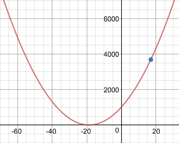
\[ \begin{eqnarray*} \alignTwoEqs{e}{(g - a)^2} \alignTwoEqs{e}{((1.8 \times C + 32) - (0.1 \times C + 0.2))^2} \alignTwoEqs{e}{(1.7 \times C + 31.8)^2} \alignTwoEqs{e}{2.89 \times C^2 + 108.12 \times C + 1011.24} \end{eqnarray*} \]
With the mean squared error, we see that the slope is much steeper further away from zero error, but it starts to flatten out as the error approaches zero. It behaves just like it looks: If we could place a ball at the top of the slope, it'd fall quickly toward zero, but if we placed a ball very close to the bottom of the valley, then it'd roll much slower. Similarly, the closer the error is to zero, the smaller the change in the weight.
So how does this new formula affect the blame we assign each weight? How do their derivatives change? Remembering our chain rule,
\[ \frac{\partial e}{\partial w} = \frac{\partial e_{mse}}{\partial e_{simple}} \frac{\partial e_{simple}}{\partial a} \frac{\partial a}{\partial w} \]
we calculate:
\[ \begin{eqnarray*} \alignThreeEqs{ \frac{\partial e_{mse}}{\partial e_{simple}} }{ \frac{\partial}{\partial e_{simple}}(e_{simple})^2 }{ 2 \times e_{simple} } \end{eqnarray*} \]
Conveniently, the remaining derivatives remain unchanged.
\[ \begin{eqnarray*} \alignThreeEqs{ \frac{\partial e_{simple}}{\partial a} }{ \frac{\partial}{\partial a} (g - a) }{ -1 } \end{eqnarray*} \]
\[ \begin{eqnarray*} \alignThreeEqs{ \frac{\partial a}{\partial w_1} }{ \frac{\partial}{\partial w_1}(w_1 \times input + w_2) }{ input }\\ \alignThreeEqs{ \frac{\partial a}{\partial w_2} }{ \space\space \frac{\partial}{\partial w_2}(w_1 \times input + w_2) }{ 1 } \end{eqnarray*} \]
Like last time, we solve for \(e\)'s derivative with respect to each weight.
\[ \begin{eqnarray*} e_{w1}'(input, e_{simple}) & = \alignThreeEqs{ \frac{\partial e}{\partial w_1} }{ (2 \times e_{simple})(-1)(input) }{ -2 \times e_{simple} \times input }\\ e_{w2}'(1, e_{simple}) & = \alignThreeEqs{ \frac{\partial e}{\partial w_2} }{ (2 \times e_{simple})(-1)(1) }{ -2 \times e_{simple} } \end{eqnarray*} \]
You may sometimes see the MSE calculated without multiplying \(e_{simple}\) by 2. This is done by defining the error function as \(\frac{1}{2}(g - a)^2\), so that the 2s in the derivative will cancel out altogether.\(^1\) Tensorflow's implementation of MSE, however, does not simplify with \(\frac{1}{2}\), so we'll be leaving the 2 in our derivative as well. (Initially, the thought of willy-nilly adding or removing a 2 made me very uncomfortable, but in fact, our network already scales everything by a learning rate anyway, so any additional linear scale doesn't matter.)
Unlike in Chapter 1, \(e_w'\) is a function of both \(e_{simple}\) and the neuron's \(input\) to update the weight's value. So with MSE, the amount we update each weight is a function of more than just \(e_{simple}\).
Looking at our neuron's formula \(input \times w_1 + w_2\), we see that no matter what the value of \(input\) is, only the first half of the formula is affected \((input \times w_1)\), and the second half of the formula is always the same \((w_2)\). Similarly, when we calculate adjustments to our weights, the \(input\) should only affect the adjustment the first weight \(w_1\) and not the second weight \(w_2\). We'll talk more about this in Chapter 3.
Updating our code to implement MSE is straight forward. The only changes to our Neuron class are the formula in errorFor() and the e_deriv portion of the derivative functions:
    function errorFor(goal){
        return pow(simpleErrorFor(goal), 2)         // updated
    }

    function errorDerivativeForWeight0(e_simple){
        e_deriv = 2 * e_simple                      // updated
        e_simple_deriv = -1
        a_deriv = input
        return e_deriv * e_simple_deriv * a_deriv
    }

    function errorDerivativeForWeight1(e_simple){
        e_deriv = 2 * e_simple                      // updated
        e_simple_deriv = -1
        a_deriv = 1
        return e_deriv * e_simple_deriv * a_deriv
    }
Those three lines are all that's needed to swap out our old error measure for our new mean squared error.
So is this new error measurement better than our original one? Let's find out how a new error formula affects how fast we can train our network. When we used \(\big|e_{simple}\big|\) for our error calculation in Chapter 1, it took us 3600 training iterations until our neuron could predict within \(\frac{1}{2}\) a degree. I've added a rolling average calculation to our training code below, so let's find out how many iterations our updated neuron will take to train.
n = new Neuron()

for(iter = 1 ... 3600){
    celsius = random() % 20 - 10
    fahrenheit = 1.8 * celsius + 32

    n.input = celsius
    n.feedForward()
    n.backpropagate(fahrenheit)

    avgError = avgError * 0.99 + abs(n.errorFor(y)) * 0.01

    if(avgError < .25){
        log("Error is less than 0.25 degrees at iteration %", iter)
        break
    }
}So far we've been defining \(e_{simple} = (g - a)\), but in some places you'll see error defined as \(e_{simple} = (a - g)\). How does defining \(e_{simple}\) in this opposite way affect the adjustments to our weight? Let's recalculate the derivatives for MSE using this new \((a - g)\) measure for error, which we'll call \(e_{flipped}\).
\[ \begin{eqnarray*} \alignThreeEqs{ e_{flipped} \vphantom{\frac{\partial e_{mse}}{\partial e_{flipped}}} }{ a - g }{ -e_{simple} } \end{eqnarray*} \]
This flips the sign of our error, does it also flip the sign of our adjustment? Why or why not?
\[ \begin{eqnarray*} \alignThreeEqs{ \frac{\partial e_{mse}}{\partial e_{flipped}} }{ \frac{\partial}{\partial e_{flipped}}(e_{flipped})^2 }{ 2 \times e_{flipped} }\\ \alignThreeEqs{ \frac{\partial e_{flipped}}{\partial a} }{ \frac{\partial}{\partial a} (a - g) }{ 1 \tag{different} }\\ \alignThreeEqs{ \frac{\partial a}{\partial w_1} }{ \frac{\partial}{\partial w_1}(w_1 \times input + w_2) }{ input }\\ \alignThreeEqs{ \frac{\partial a}{\partial w_2} }{ \space\space \frac{\partial}{\partial w_2}(w_1 \times input + w_2) }{ 1 } \end{eqnarray*} \]
And now we see that the adjustments to our weights are flipped as well, but remember that the sign of \(e_{simple}\) has flipped as well, so our weights are changed by the same amount in the same direction.
\[ \begin{eqnarray*} e_{w1}'(input, e_{flipped}) &=& \frac{\partial e}{\partial w_1} &=& (2 \times e_{flipped})(1)(input)\\ &\vphantom{\frac{\partial e}{\partial w_1}}& &=& 2 \times e_{flipped} \times input\\ &\vphantom{\frac{\partial e}{\partial w_1}}& &=& -2 \times e_{simple} \times input \tag{same!}\\ e_{w2}'(1, e_{flipped}) &=& \frac{\partial e}{\partial w_2} &=& (2 \times e_{flipped})(1)(1)\\ &\vphantom{\frac{\partial e}{\partial w_1}}& &=& 2 \times e_{flipped}\\ &\vphantom{\frac{\partial e}{\partial w_1}}& &=& -2 \times e_{simple} \tag{same!}\\ \end{eqnarray*} \]
So if you ever see error definitions using \(a - g\) instead of \(g - a\), you can rest easy that all of the math works out exactly the same. Our neuron's weights will be updated the same direction either way.
As I was first learning about neural networks, it was at this point that things really started to make sense from the math perspective, but I was still unsure from the code perspective.
Most tutorials either used a library like Keras that had already separated error from activation, or by building a bare bones python network that had the error formula baked in and unchangeable, as we've done so far.
Specifically, in our case, the error calculations in errorDerivativeForWeight are tied much too tightly to the neuron itself.
    function errorDerivativeForWeight0(e_simple){
        e_deriv = 2 * e_simple // updated
        e_simple_deriv = -1
        a_deriv = input
        return e_deriv * e_simple_deriv * a_deriv
    }
It's convenient for the neuron to calculate its own error from a goal, and then to calculate its own e_deriv, but it makes it much harder to hot-swap out different error methods to see how they behave.
Ideally, the error calculations would be factored out from the neuron's code, and it wasn't immediately clear which pieces of that function should stay in the neuron, if any, and which would be pulled out into an Error class.
Looking at the math again, we can separate out the forward propagation into two sections: everything up to the neuron's activation (the weights, input, and neuron formula), and everything after the neuron's activation (the simple error and final error).
\[ \underbrace{ w, i \Rightarrow a }_{\text{neuron}} \Rightarrow \underbrace{ e_{simple} \Rightarrow e_{final} }_{\text{error}} \]
For backpropagation, we align these same responsibilities to their derivatives. Since we are splitting \(\frac{\partial e}{\partial w}\) into parts with the chain rule, the error function is responsible for the first part \(\frac{\partial e}{\partial a}\), and the neuron is responsible for calculating the last part \(\frac{\partial a}{\partial w}\).
\[ \begin{equation} \frac{\partial e}{\partial w} = \underbrace{ \frac{\partial e_{final}}{\partial e_{simple}} \frac{\partial e_{simple}}{\partial a} }_{\text{error}} \, \underbrace{ \vphantom{\frac{\partial e_{final}}{\partial e_{simple}}} \,\, \times \frac{\partial a}{\partial w} \,\, }_{\text{neuron}} \end{equation} \]
For us to be able to swap out error implementations, the derivative \(\frac{\partial e}{\partial a}\) that we calculate in e_deriv should be handled outside of the neuron, and \(\frac{\partial a}{\partial w}\) from a_deriv onward should stay inside the neuron. Our neuron shouldn't care at all about how the error's derivative was calculated, it only needs to know the final derivative.
In that separation above, the neuron needs to know about \(\frac{\partial e_{final}}{\partial a}\), and then it can calculate its own \(\frac{\partial a}{\partial w}\) and apply that error to each weight.
In code, this separation of responsibilities looks like:
    // Somewhere else, outside the Neuron class
    e_final_deriv = 2 * e_simple
    e_simple_deriv = -1
    e_deriv = e_final_deriv * e_simple_deriv

    // a much simpler function for the neuron
    function errorDerivativeForWeight0(e_deriv){
        a_deriv = input
        return e_deriv * a_deriv
    }
So our future error calculator will calculate e_deriv, and our neuron will still calculate a_deriv. That's the correct separation of powers, as the neuron controls its activation, so it should control the \(\frac{\partial a}{\partial w}\), and the error calculator handles calculating error from activation, so it should handle \(\frac{\partial e}{\partial a}\).
Currently, our neuron's code contains 100% of the formulas that make the neural network work. Just as we've done in the math formulas above, I find it very helpful to separate out the error function from the neuron in our code too. This way, I can think of our \(a = w_1i + w_2\) neuron separately from our \((e_{simple})^2\) or \(\big|e_{simple}\big|\) error functions, whereas right now all of that code is jumbled into the same class.
Let's start by pull the errors out into their own classes. Each error option should be able to calculate its absolute error and its derivative with respect to activation, so we'll only need those two functions for each error.
abstract class SimpleError{
    function error(goal, activation){
        return goal - activation
    }
    function derivative(goal, activation){
        return -1
    }
}

class ABSError : SimpleError{
    function error(goal, activation){
        return abs(super.error(goal, activation))
    }

    function derivative(goal, activation){
        derivSimpleError = super.derivative(goal, activation)
        if (super.error(goal, activation) > 0) {
            derivABS = 1
        } else {
            derivABS = -1
        }
        return derivABS * derivSimpleError
    }
}

class MSEError : SimpleError{
    function error(goal, activation){
        simpleErr = super.error(goal, activation)
        return simpleErr * simpleErr
    }

    function derivative(goal, activation){
        derivSimpleError = super.derivative(goal, activation)
        derivMSE = 2 * super.error(goal, activation)
        return derivMSE * derivSimpleError
    }
}
Looking at these error classes, it's easier to see the requirements for building even more error functions: we need to calculate the error given a goal and activation, and also be able to compute its derivative with the same inputs. As long as we can compute the total error and derivative with just a goal and activation as inputs, then we have enough to build a new error function.
Now that we have our error functions separated out into their own classes. Let's update our neuron class to use these error classes instead of calculating its own error.
class Neuron{
    property input
    property activation
    property weights = [0.1, 0.2]
    property learningRate = 0.01

    function feedForward(){
        activation = weights[0] * input + weights[1]
        return activation
    }

    function backpropagate(e_deriv){
        delta_w0 = errorDerivativeForWeight0(e_deriv)
        delta_w1 = errorDerivativeForWeight1(e_deriv)
        weights[0] -= learningRate * delta_w0
        weights[1] -= learningRate * delta_w1
    }

    function errorDerivativeForWeight0(e_deriv){
        a_deriv = input
        return e_deriv * a_deriv
    }

    function errorDerivativeForWeight1(e_deriv){
        a_deriv = 1
        return e_deriv * e_simple_deriv * a_deriv
    }
}
These new error classes and updated Neuron class let us easily swap out the error method used during training.
n = new Neuron()
n = new Neuron()
errCalc = MSEError.singleton
// or errCalc = ABSError.singleton

for(1 ... 3600){
    celsius = random() % 20 - 10
    fahrenheit = 1.8 * celsius + 32

    n.input = celsius
    n.feedForward()

    e_deriv = errCalc.derivative(fahrenheit, n.activation)
    n.backpropagate(e_deriv)

    log("Asked for %℃ => %℉. Predicted %℉. Error %",
        celsius, fahrenheit, n. activation, error)
}
That's all we need to do to change how we calculate a neuron's error. Next, we'll start looking at different kinds of neurons. So far we've only seen linear neurons \(w_1i + w_2\), but in Chapter 3 we'll look into non-linear neurons.
Thanks for reading! I'd love to know what you thought of Chapter 1 and 2, and what you'd like to see in upcoming chapters. Please send me your feedback at adam@milestonemade.com.
And if you haven't already, sign up at https://www.milestonemade.com/building-with-neurons/ to be notified when new chapters are available!